2. Quick start¶

2.1. Project Structure¶

PyCellID is an Open Source python package designed for recursively navigating a path and tracking down data tables and metadata (mapping), returning a unique CellData object. It relates easily the data with the associated images.

The power of PycellID will be maximized when working with images of time series.

file structure:

~folder_location
|
|--- my_experiment/
     |
     |---Position01/
     |   |---mapping.txt
     |   |---out_all.txt
     |   |
     |---Position02/
     |   |--- ...
     |   |
     |---Position03/
     |   |--- ...
     |   |
     |---Position32/
     |   |--- ...
     |   |
     |---channel-x_Position01_time01.tif
     |---channel-x_Position01_time01.tif.out.tif
     |--- ...
     |---channel-z_PositionW_timeY.tif

2.1.1. Resource helpers¶

[1]:

# Build or load your data, inspect your images and make plots.
from pycellid.core import CellData, CellsPloter
# Build or load data frame.
import pycellid.io as ld
# Get a 2-D aray representing your images.
from pycellid import images
import matplotlib.pyplot as plt

2.2. Load your data¶

2.2.1. Load your data frame¶

Instantiate a CellData from your data table and the path to your images.

2.2.2. From Cell-ID output¶

[2]:

df = CellData.from_csv('samples_cellid')

[3]:

display(df)

	pos	t_frame	ucid	cellID	time	xpos	ypos	a_tot	num_pix	fft_stat	...	f_nucl_tag6_tfp	f_nucl_tag6_yfp	f_local_bg_cfp	f_local_bg_rfp	f_local_bg_tfp	f_local_bg_yfp	f_local2_bg_cfp	f_local2_bg_rfp	f_local2_bg_tfp	f_local2_bg_yfp
0	1	0	100000000000	0	0	29	725	527.0	527	0.387982	...	1675334.0	54200.0	378.6183	240.4300	12571.83	312.5942	372.9697	241.2194	12523.050	310.0760
1	1	1	100000000000	0	0	31	725	614.0	614	0.443545	...	1473843.0	54020.0	383.6143	240.4676	12212.17	319.5286	377.4458	240.1235	12138.300	317.3976
2	1	2	100000000000	0	0	31	724	639.0	639	0.500724	...	1451150.0	46463.0	379.6064	241.2868	11988.62	322.5431	376.9560	242.0784	11993.090	323.3418
3	1	3	100000000000	0	0	31	725	688.0	688	0.591332	...	1566434.0	47871.0	390.2697	436.6727	11646.41	330.3378	391.3493	437.9252	11549.440	331.3429
4	1	4	100000000000	0	0	24	721	457.0	457	0.085026	...	1204067.0	52761.0	372.6058	241.3909	11593.46	330.6237	367.9105	242.5352	11503.960	329.0977
...	...	...	...	...	...	...	...	...	...	...	...	...	...	...	...	...	...	...	...	...	...
18184	3	12	300000000720	720	0	802	736	147.0	147	0.556508	...	1237009.0	39586.0	520.8205	254.4151	10049.78	612.9800	522.1818	254.9767	10533.790	621.8302
18185	3	12	300000000721	721	0	840	707	391.0	391	0.040324	...	1053566.0	44035.0	477.8000	248.6977	11320.68	576.1446	463.5887	250.3025	11368.400	571.9272
18186	3	12	300000000722	722	0	915	827	587.0	587	0.672861	...	1534440.0	58636.0	508.6136	250.6716	9132.60	578.7262	509.0000	250.9851	9129.724	572.0000
18187	3	12	300000000723	723	0	986	336	119.0	119	0.494793	...	469596.0	36213.0	530.8571	250.7143	11290.47	423.6049	536.5789	251.0638	11238.870	423.4595
18188	3	12	300000000724	724	0	1014	84	120.0	120	0.827304	...	526434.0	127674.0	453.5542	249.6765	10899.60	716.8197	460.7500	248.6575	11796.740	903.9592

PyCellID.core.CellData - 18189 rows x 125 columns

2.3. Inspect your data¶

The development team decided to use pandas library as backend because of its syntax and its extensive documentation. The idea is to make you feel you are working with a pandas object, but with the flexibility of having access to your experimental images.

You would be able to choose from different backends in future versions.

[4]:

df.describe()

[4]:

	pos	t_frame	ucid	cellID	time	xpos	ypos	a_tot	num_pix	fft_stat	...	f_nucl_tag6_tfp	f_nucl_tag6_yfp	f_local_bg_cfp	f_local_bg_rfp	f_local_bg_tfp	f_local_bg_yfp	f_local2_bg_cfp	f_local2_bg_rfp	f_local2_bg_tfp	f_local2_bg_yfp
count	18189.000000	18189.000000	1.818900e+04	18189.000000	18189.0	18189.000000	18189.000000	18189.000000	18189.000000	18189.000000	...	1.818900e+04	1.818900e+04	18189.000000	18189.000000	18189.000000	18189.000000	18189.000000	18189.000000	18189.000000	18189.000000
mean	1.966078	6.216944	1.966078e+11	317.438947	0.0	683.000935	529.324097	441.458959	441.460718	0.265314	...	1.258965e+06	1.087345e+05	462.553463	258.523334	11753.645404	502.869092	459.888134	258.526309	11921.632917	489.371202
std	0.793782	3.726506	7.937819e+10	204.508054	0.0	396.587704	289.357639	241.039776	241.038580	0.225960	...	4.217068e+05	1.837672e+05	42.853657	50.494524	1378.053509	349.180950	44.225006	50.631219	1297.764306	308.290503
min	1.000000	0.000000	1.000000e+11	0.000000	0.0	9.000000	9.000000	98.000000	98.000000	0.018116	...	2.100890e+05	7.107000e+03	314.227900	232.300000	6984.529000	0.000000	316.946400	231.608700	0.000000	0.000000
25%	1.000000	3.000000	1.000000e+11	150.000000	0.0	327.000000	285.000000	277.000000	277.000000	0.068958	...	9.154950e+05	2.818300e+04	439.835400	244.754400	10809.180000	350.870100	435.564800	244.753600	11063.320000	351.651900
50%	2.000000	6.000000	2.000000e+11	297.000000	0.0	681.000000	538.000000	384.000000	384.000000	0.202481	...	1.177204e+06	4.325000e+04	463.130400	248.077800	11783.600000	397.611100	458.925400	248.076900	11939.820000	397.530600
75%	3.000000	9.000000	3.000000e+11	452.000000	0.0	1025.000000	779.000000	555.000000	555.000000	0.420594	...	1.592472e+06	1.144470e+05	486.517200	251.027400	12781.720000	511.681500	484.095600	250.980100	12887.200000	501.397500
max	3.000000	12.000000	3.000000e+11	966.000000	0.0	1384.000000	1032.000000	1499.000000	1499.000000	2.200194	...	2.342580e+06	2.358444e+06	734.365400	615.073200	15438.730000	6654.856000	971.200000	618.813700	15294.890000	7044.286000

8 rows × 125 columns

2.3.1. Using Cell-ID features¶

2.4. Cell-ID together with PyCellID provide 5 categories of calculated variables:¶

1. General measurments.

pos,
cellID,
ucid,
t_frame,
time,
xpos,
ypos,
f_tot,
a_tot,
fft_stat,
perim,
maj_axis,
min_axis,
flag,
rot_vol,
con_vol,
a_vacuole,
f_bg

2. To calculate membrane proximal fluorescence (for relocalization experiment).

f_tot_p1_channels,
a_tot_p1,
f_tot_m1_channels,
a_tot_m1,x
f_tot_m2_channels,
a_tot_m2,
f_tot_m3_channels,
a_tot_m3

3. Information obtained from “nuclear image” type (Variables containing the area and fluorescence of concentric disks of user-defined radius).

f_nucl_channels,
f_nucl1_channels to f_nucl6_channels,
a_nucl1 to a_nucl6,
f_nucl_tag1_channels to f_nucl_tag6_channels

4. More background information.

f_local_bg_channels,
a_local_bg,
a_local,
f_local2_bg_channels,
a_local2_bg,
a_local2

5. More volume measurments.

a_surf, sphere_vol,

the final tag _channels indicates that the vatiable will be repeated for each illumination type.

For detailed information, reading Cell-ID documentation is recomended.

[5]:

df.plot()

[5]:

<AxesSubplot:>

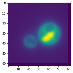
2.4.1. View your images¶

Obtain a numpy array representation of an image. Make a crop, operate o simply plot it.

[6]:

img = plt.imread("samples_cellid/YFP_Position01_time01.tif")

array = images.box_img(im=img, x_pos=640, y_pos=560, radius=30, mark_center=False)

array

[6]:

array([[371., 348., 330., ...,   0.,   0.,   0.],
       [368., 351., 368., ...,   0.,   0.,   0.],
       [370., 363., 351., ...,   0.,   0.,   0.],
       ...,
       [  0.,   0.,   0., ...,   0.,   0.,   0.],
       [  0.,   0.,   0., ...,   0.,   0.,   0.],
       [  0.,   0.,   0., ...,   0.,   0.,   0.]])

[7]:

plt.imshow(array)

[7]:

<matplotlib.image.AxesImage at 0xb50faf0>

You can use PycellID accessor to inspect images. + Use data from your dataframe for finding what you are looking for.

[8]:

# Specify your values.
df.plot(array_img_kws={"channel":"tfp", "n":50, "criteria":{"a_tot":[0, 500]}})

[8]:

<AxesSubplot:>

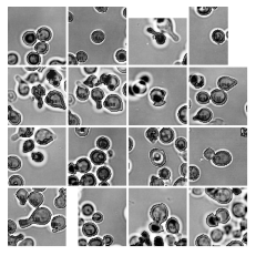
2.4.2. Use CellsPloter to inspect images¶

[9]:

cells = CellsPloter(df)

[10]:

cells.cells_image()

[10]:

<AxesSubplot:>